To enhance the capabilities of apps, one of the main side projects that I’ve been working on in between other major distractions is a framework for building and applying models that correlate chemical structure with physical properties or biological activities. The ability to apply a model, and even better to build one then make use of it, has been introduced to the SAR Table app. The underlying machinery for that particular feature is not very friendly toward larger datasets (where large means more than about a hundred compounds in this context), but there has been considerable progress in that regard, which happened to involve creating a more conventional desktop user interface, shown above.

The first premise of this model building effort is that the building process should be a black box. There are two use case scenarios: automated rebuilding from larger datasets running unsupervised, and building at the behest of an app calling a webservice, with a user interface that basically consists of a button labelled “Build Model”, i.e. also unsupervised. The second premise is that the method should be very generic: no selection of relatively arbitrary collections of so-called “2D” descriptors.

Instead, it’s all done using linear group contributions. A model is a collection of substructure fragments, and for each occurrence, the property value is incremented by the group’s assigned contribution value. It’s a very simple concept, and it has been around since the early days of cheminformatics. As far as I can tell, it’s not the most fashionable method, possibly because it seemed to outlive its usefulness for some of the more difficult properties. But I for one have always liked the idea, which could have something to do with having been a real actual chemist in a past life: if the descriptor is a chemical structure of some sort, I can convince myself that it means something to me.

So the modelling process starts by executing an efficient algorithm for finding every single subgraph of sizes from 1 to 6, where ring junctions are not included, which makes for 13 different types of graphs. Each one is further classified by element and bond orders, with a special type for aromatic bonds, and elements that are out of the common organic subset are grouped together in a smaller number of blocs. For a collection of several thousand mostly organic compounds, this will produce about ten thousand or so unique descriptors. Rather a lot, and more importantly, too many, because the model would suffer horribly from overfitting.

Now, one of the really nice features of chemical fragments is that they are not only interpretable by a human chemist, but they are also amenable to algorithmic manipulation. In particular, if you have too many chemical subgraph descriptors, no problem: they can be merged together, to create a query form.

For instance, consider the SMILES-esque representations of two descriptors:

C-C-C(=O)-C-Cl

C=C-C(=O)-C-Br

These could be merged together into a query-style descriptor which subsumes contributions from both types:

C[-=]C-C(=O)-C-[ClBr]

By judicious merging of descriptors that have similarly generic contributions to whatever property is being modelled, we can keep assimilating fingerprints until eventually we end up with a much smaller set that can provide good predictivity without overfitting.

But this creates a rather interesting optimisation problem. While it is common for QSAR model building to throw away descriptors that are not pulling their weight, I’ve not heard of a process that involves attempting to merge the descriptors together. Finding a global optimum for descriptor contributions is hard enough, but this adds an additional exponential combinatorial search space for finding out what the best descriptor combinations actually are.

The first attempt that I tried uses a genetic algorithm for searching through the space of possible contribution values, and at certain checkpoints reduces the descriptor counts by merging, with a semi-random ingredient. This actually works quite well for small datasets, up to the sizes that are well handled by the SAR Table app, and so this is currently provided as a webservice. Unfortunately it doesn’t scale well at all, and feeding in a thousand compounds chokes a modern workstation. One of the side effects of doing so much development lately for constrained mobile devices, and webservices that are expected to complete in seconds, is that I started to think of regular computers running overnight batch tasks as having infinite resources available to them. They don’t, and a genetic algorithm coupled with a lot of extra degrees of freedom exceeds the acceptable conditions.

It turns out that running a much simpler single-point refinement process works quite well, too. Instead of spawning a large population of possible solutions, a single proposed solution is perturbed then re-solved for each of its descriptors, using a little bit of calculus and a heavy helping of brute force. Even with a single refinement point, though, the matrix of total descriptors x total responses is excessive, and so in the interests of getting the job done in a reasonable length of time, the refinement starts with only the few hundred most popular descriptors. The rest have to sit out on the sidelines (the “reserve”). Each time the iteration converges, one of the reserve descriptors is picked. This causes the total descriptor count to exceed the limit, and so the algorithm goes hunting for two descriptors that can be merged together: it tests each combination, and goes with the one that can be accomplished with the least reduction of the score. And so on, until the total number of descriptors is below the threshold, and the model has converged.

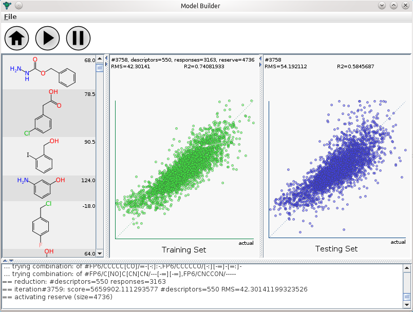
The initial method development was done using a command line tool, using the com.mmi libraries (Java). Watching text being written onscreen is not the best way to comprehend how well a model building operation is performing, and since these things can take hours, it’s very useful to get visual feedback. Which brings me back to the screenshot at the top of this post: it’s the first application I’ve written for a regular desktop interface in more than three years. The three main panels show the molecules that go into the training set, the correlation plot for the training set (green dots), and the correlation plot for the testing set (blue dots). Being able to visually observe both the training & testing set as they evolve provides a great deal of real time comfort that the model is going to have some degree of relevance when applied to data in the wild.

The desktop application may become available as a commercial product somewhere down the line, though so far it’s insufficiently complete to be let out of the lab. The screenshot in this post shows my first attempt to model a collection of relatively well curated melting point records, which are from the same data source as used by the Open Notebook Science melting point predictions. Melting points are notoriously hard to model, but it turns out that this may be because the source data is usually so terrible. Much better results can be obtained from cleaned up data, and the rationale for using the group contribution method is that many of the descriptors that go into the better models are themselves derived from methods that are quite similar to group contributions… so maybe cutting out the middle man will add a little boost. Or at least break even, and allow models that are just as good to be built with little or no special tweaking.

The log P model is already in quite good shape, and comparisons with the test set indicate that it’s working at least as well as what passed for state of the art ten years ago. Which means that the current log P calculator used by several apps – based on a method more than ten years old – will be replaced with this one.