Some interesting experimental features are on their way to the Approved Drugs app, which has been in the crosshairs for expanded functionality recently. The latest round of improvements involves the ability to collect custom-drawn structures, and apply Bayesian models for predicting the presence of “bad drug” properties, both for molecules overall, and for individual atoms.

For purposes of model building, the foundational technology is the portable implementation of so-called “circular” ECFP6 fingerprints, which were developed on behalf of CDD, and subsequently ported to iOS for use in the TB Mobile app, for similarity and clustering. After a significant amount of tinkering with using these fingerprints for Bayesian models, I eventually settled on an implementation pattern and a file format that allows models to be conveniently built using a desktop computer to grind through hundreds of thousands of input structures and then exporting the distilled results into a mobile app.

Working with Bayesian models is a fairly convenient process as far as chemical modelling algorithms go, but there are a fair few gotchas. For example, knowing when and how much to “fold” fingerprints is important: collapsing into a smaller addressable range saves space and improves performance, but it introduces artifacts, i.e. when two completely different structural fragments share the same tag. Bayesian models are rather good for processing large datasets quickly (e.g. a million compounds a minute is quite realistic), but that means the implementation has to be constructed carefully so that it does not accumulate unnecessary memory allocations, or expose any scaling issues like O(N²) loops that may have gone unnoticed when testing on smaller validation sets. And then there are the issues involved with using modified Bayesian predictors that are sums of log values, which means that the numbers that come out the other end are not probabilities (0..1) like in pure Bayesian methods, but rather are unscaled numbers with no meaningful upper or lower bound, or midpoint. Deciding what value makes for a good cutoff for active vs. inactive involves a bit more voodoo than with a probability value (i.e. you can’t just use >0.5). Analysing the receiver-operator-characteristic (ROC) curve is one way to get around the calibration issues.

Without going into detail (yet) about how these issues are resolved, the bottom line is that a concise model file can be incorporated into the bundle for a mobile app, and since the MMDSLib library features calculation of the appropriate fingerprints, it is now easy to map a structure into a model prediction. One of the first demonstrations of this is in the current development version of the Approved Drugs app, which has been extended to allow users to draw their own custom structures, and select from preexisting models:

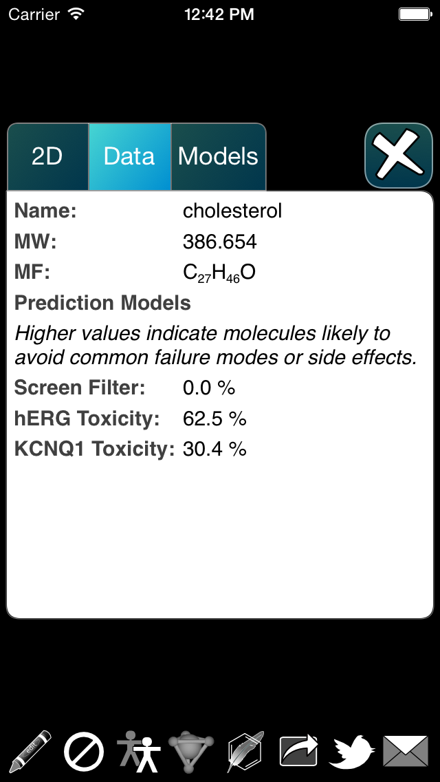
At the moment there are three models, which are abbreviated as Sf (for screening filter), hE (for hERG) and Kq (for KCNQ1). The so-called screening filter is based on output from rules designed to eliminate molecules that are not worth evaluating as potential drugs, while the other two are human targets that should generally be avoided, because any proposed drug that binds to them inadvertently is likely to fail in the clinic. The colour-coding scheme uses the common “traffic lights” colour scheme, where green is good (doesn’t hit the unwanted properties), yellow is a warning, and red means that it is rather likely to be problematic, at least as far as the model is concerned.

Rendering a single calibrated Bayesian prediction as a colour-coded property for a molecule is interesting and useful, but it’s not the last word on the matter. Because the models are built from fingerprints that have specific chemical meaning, there are additional properties. Visually, one way of representing a particular ECFP6 fingerprint is shown below:

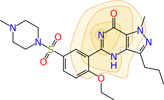
The atom that is centred at the middle of the contours is ground zero for this particular fingerprint. The full definition is created by iterating outward and adding all neighbouring atoms 3 times (hence the “diameter” of 6). In this case the fingerprint represents 11 atoms, and their subgraph is converted into a 32-bit number, which is its “hash code”. The collection of all of the hash codes for the molecule (there are typically several hundred) make up its fingerprint, and these are fed into the Bayesian model. Once the model is created, each hash code is given a contribution toward the overall prediction, of whether the molecule is active or inactive (or whatever on/off property is being modelled).

So, because each hash code has an assigned contribution, it is possible to look at an individual molecule and map each hash code to the actual atoms that were involved in the creation of that hash code. The contributions per fingerprint atom block can be summed over individual atoms, to get an indication of the relative extent to which each atom contributes positively or negatively to the overall prediction. By contemplating the overall prediction value for the molecule, and the distribution of atom contributions, it is possible come come up with a rendering that is indicative of which parts of the molecule are good or bad:

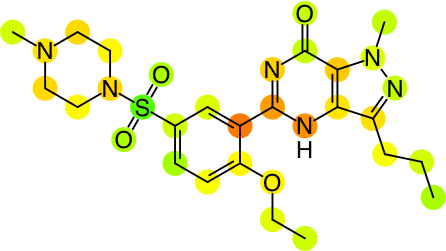
As currently implemented in the yet-to-be-released version of Approved Drugs, the predictions can be visualised for the whole collection of molecules, or for the detail view of an individual molecule:

The graphical view is currently implemented as a scrollable panel, i.e. an overlay is shown for each of the available models, which can be swiped left or right to view each one.

This new functionality is a work in progress. There are just the three models available, which are hardwired into the app: they will be supplemented and improved with further iterations, as well as properly documented at some point. While the method for using Bayesian models to estimate an overall prediction is well established science, breaking them out into individual atom contributions is not, and at the time of writing, formal validation is still on the to-do list. As it happens, coming up with a way to rigorously normalise the values is not exactly obvious, but even in its current state it does serve to provide a clear way to communiate both the overall prediction, and whether a particular region of the molecule carries more than its fair share of the credit or blame for why this is so.